Adding a mass-balance model¶

In this exemple, we demonstrate how to provide an independant mass-balance model to OGGM. The example code can be found in oggmcontrib/mbmod.py.

In order to be used by the dynamical model, the mass-balance model must comply to a relatively simple interface:

it must return the mass-balance as a function of time and altitude
it must comply yo the units needed by the ice dynamics model: meters of ice per second

The time-step at which the dynamical model requires mass-balance is a user parameter, and the current default is at annual time steps. Previous studies and experience shows that coupling the ice dynamics and mass-balance models at more frequent time steps is not necessary. It doesn’t mean, however, that the mass-balance model cannot compute the mass-balance at shorter time intervals: the interface just has to integrate the mass-balance over a year before giving it to the dynamical model.

In the provided example, we compute a linear mass-balance profile as a function of a randomly chosen equilibrium line altitude.

Apply our new model to Hintereisferner¶

Let’s apply the standard OGGM workflow to our glacier:

import geopandas as gpd
import numpy as np
import matplotlib.pyplot as plt
import oggm
from oggm import cfg, tasks
from oggm.utils import get_demo_file
from oggm import workflow

# Set up the input data for this example
cfg.initialize()
cfg.PATHS['working_dir'] = oggm.utils.get_temp_dir('oggmcontrib_mb')
cfg.PATHS['dem_file'] = get_demo_file('srtm_oetztal.tif')
cfg.PATHS['climate_file'] = get_demo_file('histalp_merged_hef.nc')
cfg.set_intersects_db(get_demo_file('rgi_intersect_oetztal.shp'))

# Set up the run parameters
cfg.PARAMS['baseline_climate'] = 'CUSTOM'
cfg.PARAMS['run_mb_calibration'] = True
cfg.PARAMS['border'] = 80
cfg.PARAMS['use_multiprocessing'] = True

# Glacier directory for Hintereisferner in Austria
entity = gpd.read_file(get_demo_file('Hintereisferner_RGI5.shp')).iloc[0]
gdir = oggm.GlacierDirectory(entity)

# The usual OGGM preprecessing
tasks.define_glacier_region(gdir, entity=entity)
workflow.gis_prepro_tasks(gdir)
workflow.climate_tasks(gdir)
workflow.inversion_tasks(gdir)
tasks.init_present_time_glacier(gdir)

This was all OGGM stuff. Now, let’s define our own model for this glacier:

In [1]: from oggmcontrib.mbmod import RandomLinearMassBalance

In [2]: mbmod = RandomLinearMassBalance(gdir, seed=0, sigma_ela=200)

The ELA will vary randomly with a standard deviation of 200 m. What does that mean for the glacier? Let’s compute the specific mass-balance integrated over the flowline glacier:

In [3]: heights, widths = gdir.get_inversion_flowline_hw()

In [4]: smb = mbmod.get_specific_mb(heights, widths, year=np.arange(50))

In [5]: plt.figure(figsize=(7, 4));

In [6]: plt.plot(smb, label='Specific MB (mm we yr$^{-1}$)');

In [7]: plt.legend();

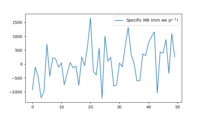
These are variations in the same order of magnitude as observed in the last 60+ years, with the difference that they are rather positive, not negative.

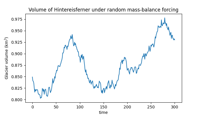
Let’s give this mass-balance model to the OGGM glacier dynamics model and run it for 300 years:

In [8]: from oggm.core.flowline import flowline_model_run

In [9]: flowline_model_run(gdir, mb_model=mbmod, ys=0, ye=300);

The model stored its output in standard NetCDF files. Let’s just have a look a it!

In [10]: import xarray as xr

In [11]: ds = xr.open_dataset(gdir.get_filepath('model_diagnostics'))

In [12]: (ds.volume_m3 * 1e-9).plot();

In [13]: plt.ylabel('Glacier volume (km$^{3}$)');

In [14]: plt.title('Volume of Hintereisferner under random mass-balance forcing');